Generating GHZ state on IBM device
A look into the final lab of IBM Quantum Spring Challenge 2023
IBM Quantum Spring Challenge 2023
IBM Quantum Spring Challenge was a public event held from May 17 to May 24. This challenge is part of IBM Quantum’s ongoing global education efforts and is free to participate in. The challenge’s goal is to provide participants with a deeper understanding of a specific quantum topic.
This year’s challenge marked the third anniversary of the IBM Quantum Challenge since May 2020. The challenge focuses on dynamic circuits, which allow for classical processing during the runtime of the circuit. The dynamic circuits were implemented in the challenge to demonstrate error mitigation and quantum teleportation. Participants also have the opportunity to run their program on a 127-qubit device.
Running a quantum algorithm in the current noisy intermediate-scale quantum (NISQ) era remained challenging due to the quality and the limited number of qubits. Thus, the hybrid quantum-classical algorithm was introduced to reduce circuit depth for NISQ devices.
127-qubit Device
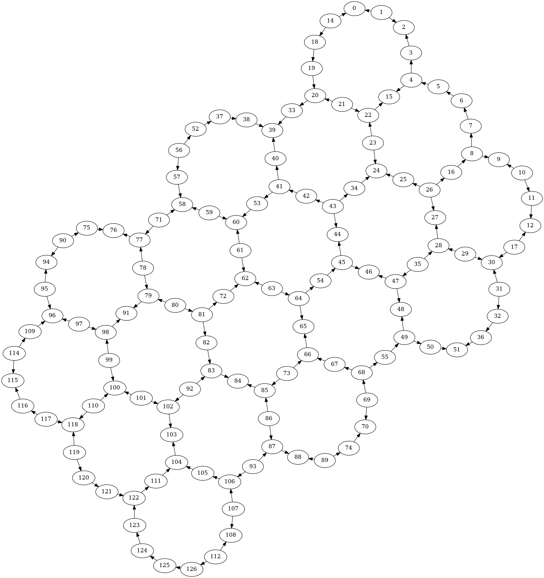
The ibm_sherbrooke system assigned to the challenge is a 127-qubit Eagle processor optimized for error mitigation. Instead of CNOT gates, unidirectional echoed cross-resonance (ECR) gates were implemented due to their simplicity and noise resilience. The coupling map of the device is shown below as a directional graph.
The implementation of these unidirectional ECR gates resulted in an interesting CNOT gate transpilation. Since CNOT gate is not a symmetric gate, the transpilation depends on the direction of the CNOT gate. Some transformation identities for assymetric gates are defined in GateDirection. Meanwhile, CNOT gate is transpiled into ECR and single qubit gate up to a global phase shift.
![]()
![]()
For instance, the unidirectional ECR gate between the qubit $q_{63}$ and $q_{64}$ is implemented in the forward direction from $q_{63}$ to $q_{64}$. The CNOT gate transpilation with control at $q_{63}$ and target at $q_{64}$ resulted in only a depth 5 circuit while depth 7 when reversed.
GHZ State
The GHZ (Greenberger–Horne–Zeilinger) state is a specific type of quantum entangled state of multiple qubits named after the physicists Daniel Greenberger, Michael Horne, and Anton Zeilinger. The GHZ state is a maximally entangled state of the form
\[\frac{1}{\sqrt{2}}\left(|0\rangle^{\otimes n}+|1\rangle^{\otimes n}\right)\]where $n$ is the number of qubits. Note that in the case of $n=1$, the equation is reduced to the Bell state. One of the intriguing properties of the GHZ state is that it exhibits perfect correlations. That is, the measurement of one qubit resulted in the same outcome for all other qubits, which is a direct consequence of quantum entanglement.
Generating a Large GHZ State with Stabilizers
In the final lab of IBM Quantum Spring Challenge 2023, participants were tasked to generate a 54-qubit GHZ state on the 127-qubit real device. Only the even-numbered qubits are used for the GHZ state while the odd-numbered qubits as the stabilzers.
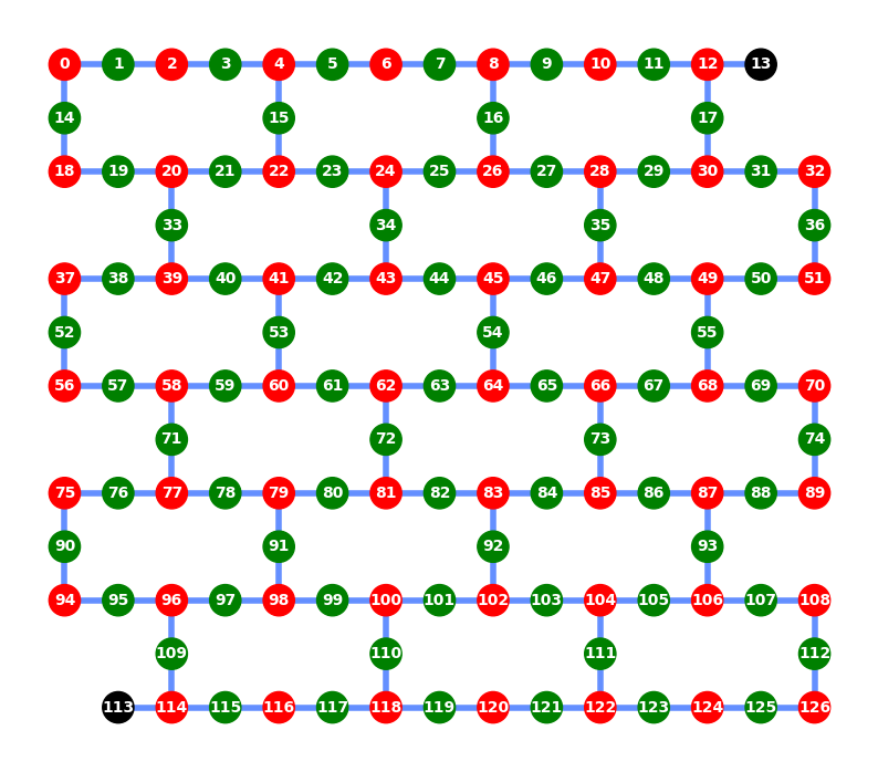
The oddness and evenness of the numbers are not to be confused (from the image, red: GHZ qubits; green: stabilizer qubits; and black: unused) with the indexing of the qubit. An unranked optional challenge to generate the GHZ state with the lowest depth can be attempted by motivated participants. Two approaches will be discussed in this post, one with $log(N)$ depth and another of constant depth with respect to the qubit size $N$.
Breadth-First Search
A GHZ state can be constructed by expanding upon the Bell state preparation circuit.
In the example, the Bell state is generated by entangling $q_0$ and $q_4$. Successive CNOT gates are then applied in parallel such that the entangled state grows as $2^d$, where $d$ is the depth of CNOT layers. In other words, the circuit depth scales with $log_2(N)$. However, this approach is limited by the actual connectivity of the device. Thus, an algorithm for generating GHZ state with stabilizers on a real device with limited connectivity is as follows:
- Identify a central node with the highest centrality
- Implement a breadth-first search (BFS) algorithm from the central node to branch out to all other nodesCNOT gates are applied in order of the branch that leads to the deepest level of the BFS tree to the shallowest
- Disentangle the stabilizer qubits
With limited connectivity, the circuit depth then scales with $log_b(N)$, where $0<b\le2$ is the branching factor.
For ibm_sherbrooke device, $q_{62}$ (node in red) was identified as one of the central nodes, and the BFS tree from this central node spans the red edges. The CNOT gates are then applied in the reversed order of depth as shown in the animation to ensure that the gate depth is bounded by the furthest node from the central node. Disentangling the stabilizer is trivial, which requires traversing the tree in reversed direction and applying a CNOT with the odd-numbered qubit as the target. However, the BFS approach is still far from optimal even when all-to-all connectivity is available.
Dynamic Circuit
In conjunction with this year’s challenge theme on dynamic circuits, an optimal solution with constant scaling can be constructed with dynamic circuits independent of the device size. First, the qubits are sorted into two groups: entangling and parity qubits by their odd-evenness, coinciding with the labeling of GHZ and stabilizer qubits. The algorithm for achieving the GHZ state is described below as:
- Apply Hadamard gate to all the entangling qubits
- Apply CNOT gate to the parity qubits using the neighboring entangling qubit as the control
- Measure all the parity qubits
- Apply the parity X gate to the qubits depending on the measurement outcome
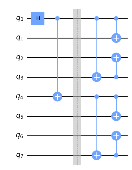
The following circuit diagram gives an example of a 3 qubit GHZ state with 2 stabilizer qubits
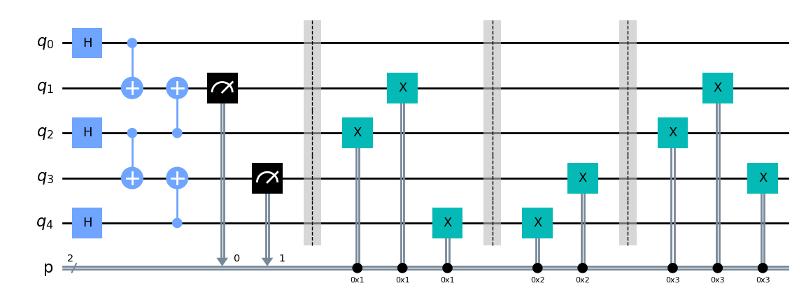
where the parity X gates are drawn explicitly using a soon-to-be deprecated c_if for clarity. The evolution of the states then follows as
Parity X gate is defined as a dynamic circuit with the following form
\[\prod_i X_{\text{ent}(i+1)}^{\oplus_i M(i)} X_{\text{partity}(i)}^{M(i)}\]Here, $M(i)$ is the measurement outcome of the $i$-th parity qubit, and $\oplus_i M(i)$ gives the modulo 2 sum of the parity qubits up til the $i$-th bit. For instance, the parity X gate acting on the $|01110\rangle=|010\rangle_{\text{ent}}|11\rangle_{\text{parity}}$ state is given by
\[X_{\text{ent}(2)} |010\rangle_{\text{ent}} \otimes X_{\text{partity}(2)} X_{\text{partity}(1)}|11\rangle_{\text{parity}} \\ = |000\rangle_{\text{ent}}|00\rangle_{\text{parity}} = |00000\rangle\]Interestingly, the parity X gate acts at most a single X gate on each qubit, yielding a depth-1 gate upon transpilation. Noting that the parity X gate depends on the parity measurement, a dynamic circuit using the switch case can be implemented.
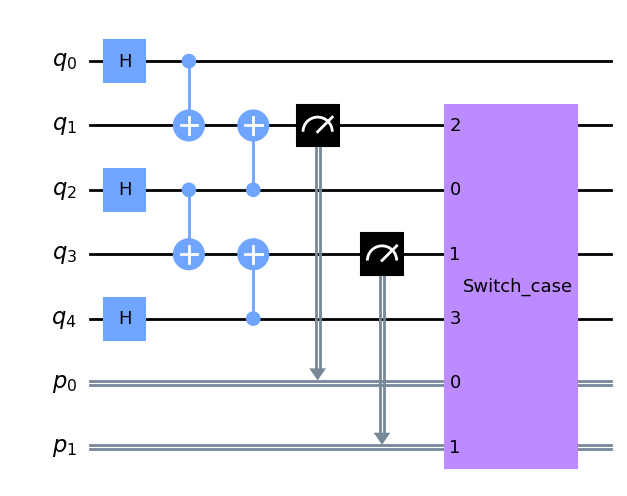
The switch/case control flow acts similarly to the switch case in most programming languages and allows for an elegant way of implementing the parity X gate. However, at the time of writing, the backend Aer 0.12.0 does not support SwitchCaseOp. So, the code implementation based on if_test and c_if are included for demonstration.
The use of dynamic circuits for GHZ generation reduced the depth required to a fixed value independent of the size, provided one can find a route that visits every node once exists. This is exactly the Hamiltonian path problem which is known to be NP-hard. In general, the Hamiltonian path is not guaranteed to exist. Instead, one can find the longest possible non-overlapping path the dynamic circuits.
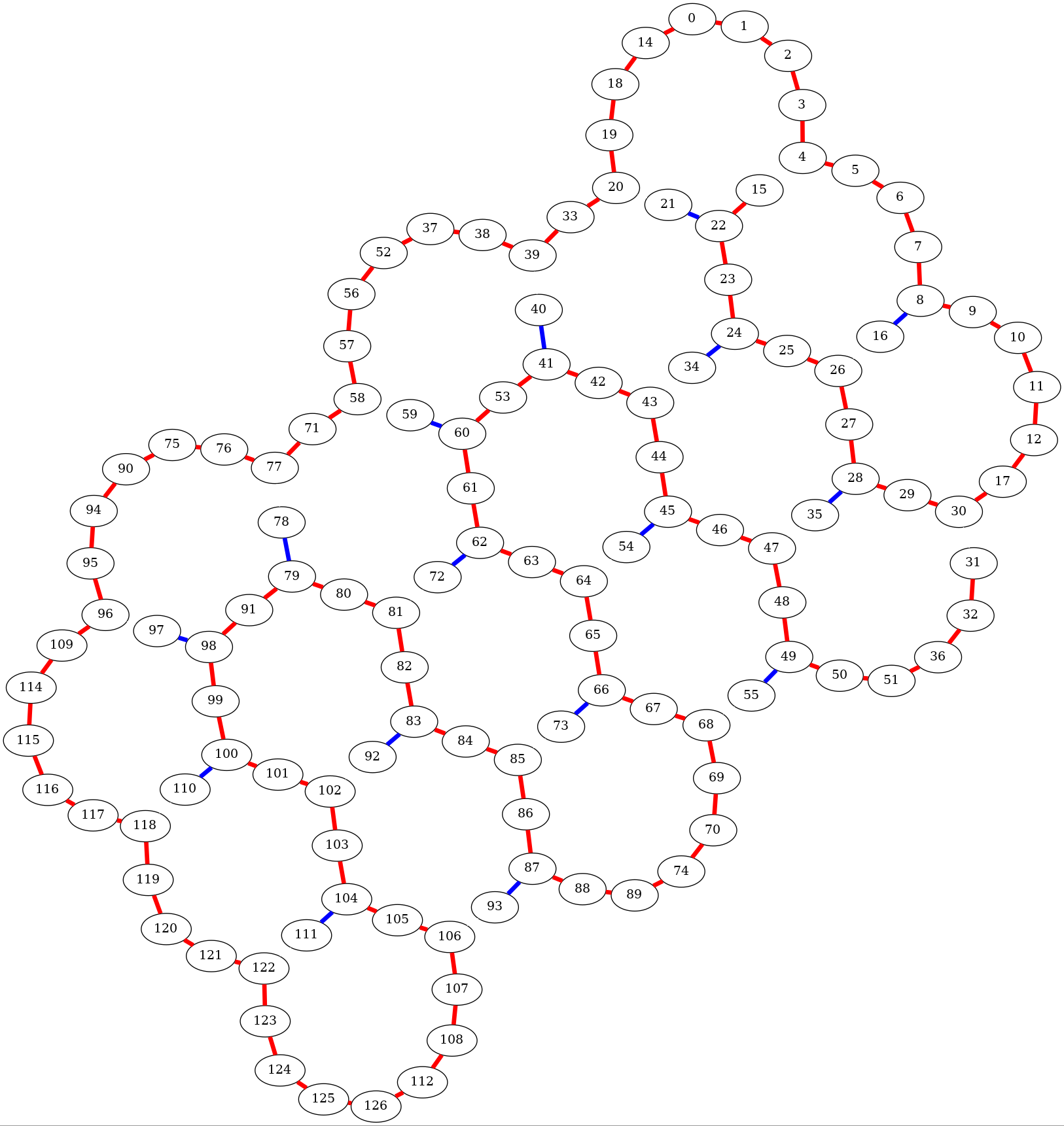
For ibm_sherbrooke, one possible solution to the longest path is shown above, tracing the red edges. Uncoupled qubits following the blue edges can then be entangled in the next step with CNOT gates, introducing an overhead of depth 1. A circuit depth of 5 is expected for the dynamic circuit scheme, plus an additional depth for the overhead, bringing to a total of 6. The application of dynamic circuits yields an optimal GHZ state with stabilizer generation with a fixed depth of 5 and a small overhead for non-ideal connectivity.
Final Remarks
The IBM Quantum Spring Challenge 2023 is an excellent opportunity for the community, beginners and professionals alike to learn about the latest development in quantum computing. Dynamic circuits being one of the new tools introduced in recent years, it would be exciting to see how they can advance the field of quantum computation. So far, this post discusses only the circuit depth reduction without considering the CNOT direction or gate error rate.