Introduction to rustworkx
With examples and applications in quantum computing
rustworkx
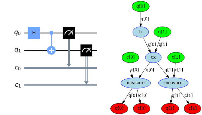
Qiskit uses rustworkx (or formerly retworkx), a graph library under the hood. rustworkx was originally conceived to build a faster directed acyclic graph (DAG) to use as the underlying data structure for qiskit-terra’s transpiler. For instance, a Bell state circuit can be represented as a directed graph as follows:
Prior to rustworkx, qiskit uses NetworkX. NetworkX’s pure Python implementation leads to a performance bottleneck, and thus rustworkx addressed this by implementing the graph data structures and algorithms in Rust. The performance gain was documented to be 3x to 100x for the same use case compared to NetworkX.
Despite basing on NetworkX, rustworkx is not a drop-in replacement, and some of its implementations varies. Key differences and conversion guide can be found here. This blog post will be looking at some of rustworkx’s features and application of a graph algorithm in quantum computing.
IBM Hardware Coupling Map
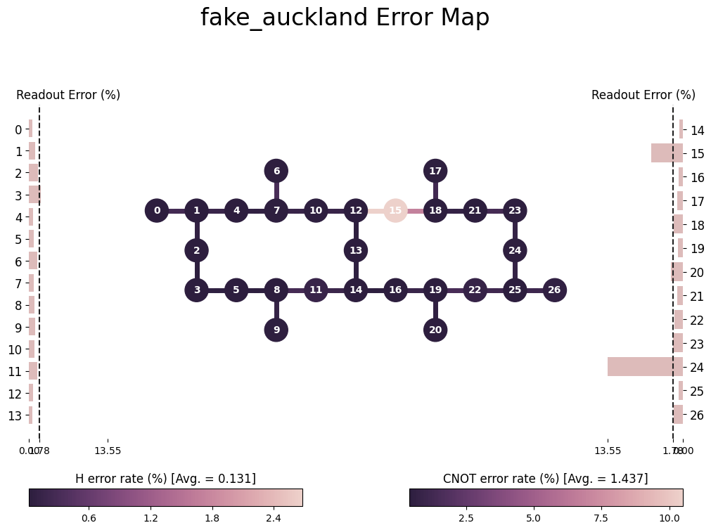
This section will use IBM’s hardware coupling map as an example to demonstrate some of rustworkx’s features. The coupling map is a graph that represents the connectivity of the qubits in a quantum device. First, the coupling map is loaded from IBM’s hardware backend:
from qiskit.providers.fake_provider import FakeAuckland

backend = FakeAuckland()
backend.coupling_map.draw()
The circles in the diagram is a node that represents a physical qubit on the device and the arrows are edges that represent the connectivity between the qubits. Each arrow has a weight that is determined by its corresponding CNOT gate error rate.
The standard graph algorithms perform summation across the edges of non-negative weights. Thus, the weights $w$ are defined as the negative log of the CNOT gate success rate:
\[w_{ij}=-\log(1-p_{ij})\]where $p_{ij}$ is the CNOT gate error rate for the control qubit $i$ and target qubit $j$. Under this convention, smaller weights correspond to higher success probability. For simplicity, the coupling map will be converted to an undirected graph because of the symmetry of the CNOT gate error rate for ibm_auckland. Special care taking into consideration of the gate asymmetry is needed for hardware such as the Eagle processor, which utilizes uni-directional echoed cross-resonance (ECR) gates.
import numpy as np
import rustworkx as rx

# extract the two-qubit error rate from the backend
two_q_error_map = {}
for gate, prop_dict in backend.target.items():
    for qargs, inst_props in prop_dict.items():
        if len(qargs) == 2:
            if inst_props.error is not None:
                two_q_error_map[qargs] = max(
                    two_q_error_map.get(qargs, 0), inst_props.error
                )

# convert two-qubit error rate to edge weight
two_q_suc = 1-np.array(list(two_q_error_map.values()))
neg_log_two_q_suc_val = -np.log(two_q_suc)
neg_log_two_q_suc = dict(zip(two_q_error_map.keys(), neg_log_two_q_suc_val))

# create undirected graph
g = rx.PyGraph(multigraph=False)
g.extend_from_weighted_edge_list([(x, y, v) for (x, y), v in neg_log_two_q_suc.items()])
An empty undirected graph PyGraph object was first created and populated with the weighted edges using extend_from_weighted_edge_list. This method will create the nodes and edges if they do not exist. The multigraph=False argument ensures that the undirected graph has no parallel edges.
Visualization
Similar to NetworkX and other popular graph packages, the generated graphs can be visualized using Matplotlib. Under rustworkx, this is done using the mpl_draw function.
from rustworkx.visualization import graphviz_draw, mpl_draw
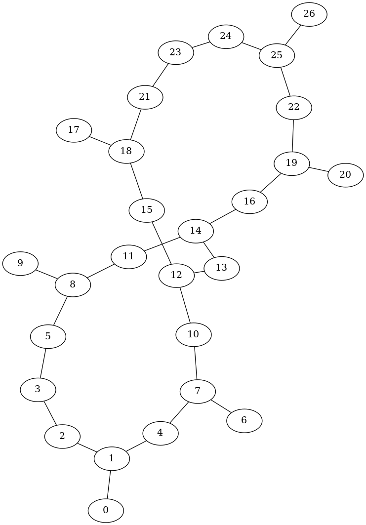
mpl_draw(g)
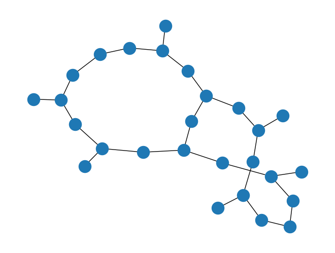
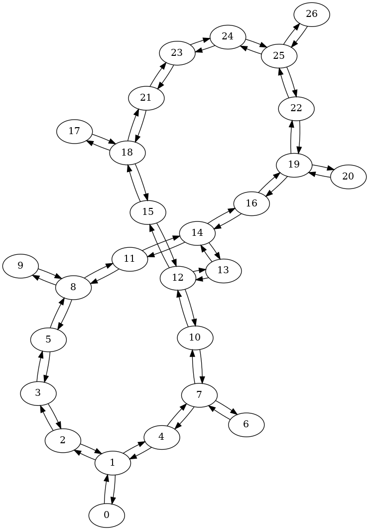
As readers may notice, using Matplotlib to visualize complex graphs can be quite cluttered. Instead, using an alternative method graphviz_draw with Graphviz to render the graph can improve the clarity and visibility of the components. Graphviz is a dedicated graph visualization software that supports detailed customization of graph styling.
graphviz_draw(g, method='neato')
Betweenness Centrality
Given the coupling map graph, it may be helpful to identify a vital node (qubit) in the graph. Centralities are measures of the relative importance of a node in a graph. One such measure is the betweenness centrality, where for each node $v$ is metric is proportional to the number of shortest paths between all pairs of nodes $\sigma(s,t)$ that passes through $v$:
\[c_B(v)=\sum_{s,t \in V}\frac{\sigma(s,t|v)}{\sigma(s,t)}\]This is available in rustworkx 0.13.0 as betweenness_centrality for only unweighted graph:
import matplotlib

# Assigning data payload to color nodes with graphviz_draw
for node_id, btw in c_degree.items():
    g[node_id] = (node_id, btw)

# Leverage matplotlib for color map
colormap = matplotlib.colormaps["magma"]
norm = matplotlib.colors.Normalize(
    vmin=min(c_degree.values()),
    vmax=max(c_degree.values())*1.2
)

def color_node(node):
    node_id, btw = node
    rgba = matplotlib.colors.to_hex(colormap(norm(btw)), keep_alpha=True)
    return {
        "color": f"\"{rgba}\"",
        "fillcolor": f"\"{rgba}\"",
        "style": "filled",
        "fontcolor": "white",
        "fontsize": "10.5",
        "label": f"{node_id}\n({btw:.2f})",
    }

graphviz_draw(g, node_attr_fn=color_node, method="neato")
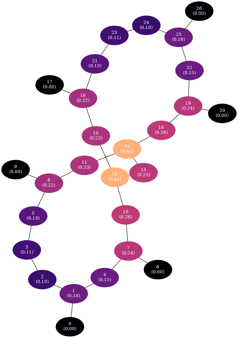
In an unweighted scenario, it appears that nodes 12 and 14 are nodes with the highest betweenness centrality. What would happen if the weight (CNOT error rates) are taken into account?
Distance Matrix
To investigate the effect of a weighted graph, the weighted variation of betweenness centrality is needed.floyd_warshall_numpy:
import matplotlib.pyplot as plt

distance_matrix = rx.floyd_warshall_numpy(g, weight_fn=float)

plt.xlabel('Node 1')
plt.ylabel('Node 2')
plt.title('Distance matrix')
plt.imshow(distance_matrix)
plt.colorbar()
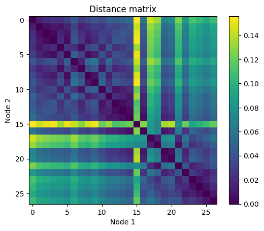
Physically, the values of each element represent the upper bound of the success probability of CNOT entangling operation between a pair of qubits.
avg_success = np.mean(np.exp(-distance_matrix), axis=1)
plt.plot(avg_success)

plt.xlabel('Node')
plt.ylabel('Average Success CNOT Entangling Probability')
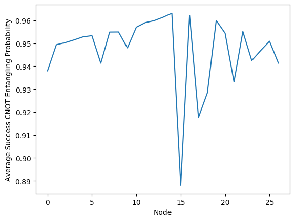
When taking into account the edge weight, the poor CNOT performance of node 15 manifests and its surrounding nodes exhibit poor average success probability. Thus, node 14 is now a better candidate for a central qubit.
Traversal
The implementation of the traversal algorithm consists of two parts: the search algorithm and the visitor object. As of rustworkx 0.13, three search algorithm with their corresponding visitor object exists:
-
dfs_search/DFSVisitor -
bfs_search/BFSVisitor -
dijkstra_search/DijkstraVisitor
The traversal algorithm of interest for the weighted graph is Dijkstra’s algorithm. The Dijkstra’s algorithm is a single-source shortest-path algorithm that is applicable to both weighted and unweighted graphs. The visitor object implements the callback functions that are invoked at each event point as defined by the pseudo-code. In particular, the event of interest is the edge_relaxed which is triggered when a shorter path is discovered. With that in mind, a visitor object that records the edges of the shortest path tree with root from the central qubit can be implemented as follows:
 class TreeEdgesRecorder(rx.visit.DijkstraVisitor):

    def __init__(self):
        self.edges = []

    def edge_relaxed(self, edge):
        self.edges.append(edge)

vis = TreeEdgesRecorder()
rx.dijkstra_search(g, [np.argmin(avg_success)], float, vis)

colormap = matplotlib.colormaps["magma"]
norm = matplotlib.colors.Normalize(
    vmin=min(avg_success),
    vmax=max(avg_success)*1.05
)

t = rx.PyDiGraph()
t.extend_from_weighted_edge_list(vis.edges)
for node_id, btw in enumerate(avg_success):
    t[node_id] = (node_id, btw)

graphviz_draw(t, method='dot', node_attr_fn=color_node, graph_attr={'rankdir': 'LR'})
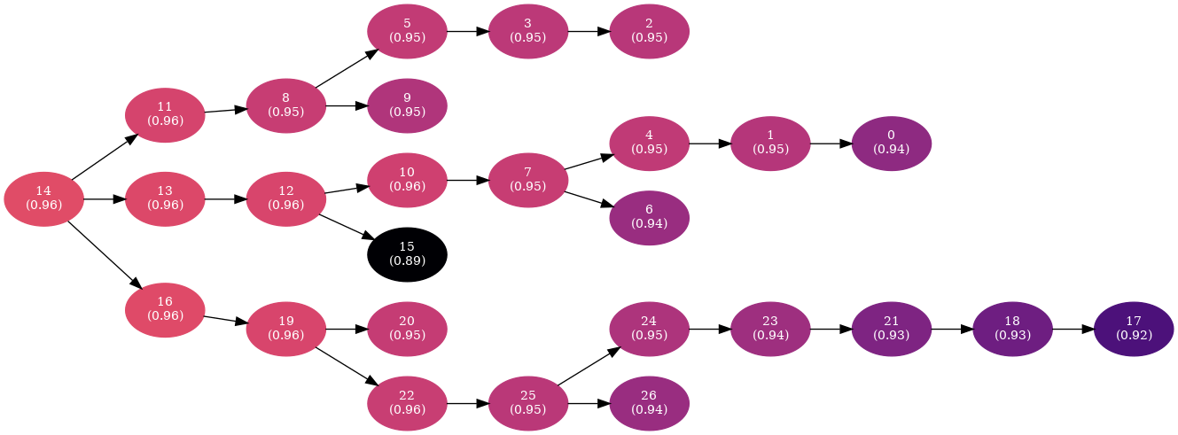
The tree obtained from the central root node provides a heuristic approach to hardware-aware mapping of quantum circuits for a whole device entanglement or state preparation (for instance, quantum circuit decomposition of a center-gauge matrix product state).
Map Coloring and Efficient Quantum Measurement
How can methods for coloring a map lead to a speedup in quantum algorithms such as variational quantum eigensolver (VQE)? This section will explore the connection between these topics and how rustworkx was used within the Qiskit codebase.
Four-Color Theorem
In the October of 1852, Francis Guthrie who was a student in London noticed that only four colors are needed to color the map of the counties of England in such a way that no two countries sharing a common border receive the same color. This then started a chain of letters which sees the birth of the four-color conjecture.
Early proofs of the theorem by Alfred Kempe in 1879 and Peter Guthrie Tait in 1880 turn out to be both fallacious after eleven years each. Eventually, the first correct proof was published in 1976 by Kenneth Appel and Wolfgang Haken. The proof was initially controversial as it was the first major theorem to be proved using a computer. Appel and Haken’s approach to proving the theorem involved reducing the infinitude of possible maps to 1834 reducible configurations which are then verified by a computer, proving that no counter-example to the four-color conjecture exists.
On any given map, each region or country on a map can be represented by a node. Two nodes are connected by an edge if the corresponding regions share a common border. Thus, the map coloring is reduced to a planar graph coloring problem. A planar graph is a graph that can be embedded in a plane without any edges crossing. For general graph coloring problems, more colors are needed.
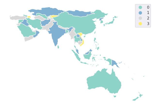
Enjoy a colored map of the Asia-Pacific!
Pauli Grouping
VQE is a hybrid quantum-classical algorithm designed to find the ground state or energy spectrum of a physical or chemical system. However, obtaining the expectation value of a Hamiltonian requires decomposition into a weighted sum of Pauli string. Each Pauli string needs to be sampled sufficiently many times to obtain a good estimate of the expectation value. Thus, the ability to simultaneously measure commuting Pauli strings, i.e. Pauli grouping is crucial to the performance of VQE.
Starting from a set of Pauli strings ["XX", "YY", "IZ", "ZZ", "ZX"], the goal is to group the Pauli strings into commuting sets. The algorithm first constructs a graph where the presence of an edge between two nodes indicates their non-commutativity. The graph is then colored such that no two adjacent nodes have the same color. The coloring of the graph then determines the grouping of the Pauli strings.
from qiskit.quantum_info import PauliList

op = PauliList(["XX", "YY", "IZ", "ZZ", "ZX"])
Coloring a graph is still an NP-hard problem, but a heuristic algorithm can be employed to obtain good coloring. The greedy algorithm is one such algorithm that is simple and fast. The algorithm starts with an empty coloring and iteratively colors the nodes with the lowest possible color. The algorithm is guaranteed to produce a coloring that is at most one more than the optimal coloring. The algorithm is implemented in rustworkx and can be accessed via graph_greedy_color.
cmap = matplotlib.cm.get_cmap('tab10')

def node_attr(node):
    rgba = matplotlib.colors.to_hex(cmap(coloring_dict[node]))
    return {'label': str(op[node].to_label()),
            'shape': 'circle',
            'fillcolor': f"\"{rgba}\"",
            'style': 'filled',
            'width': '0.9'}


graph = op._create_graph(False)
coloring_dict = rx.graph_greedy_color(graph)
graphviz_draw(graph, node_attr_fn=node_attr, graph_attr={'rankdir': 'LR'})
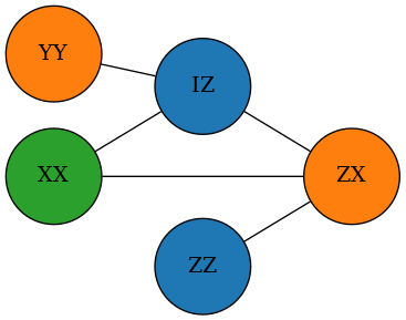
This is the exact implementation of PauliList.group_commuting under Qiskit. Now, instead of 5 measurements, only 3 measurements are needed to sample all the Pauli strings once. This is a 40% reduction in the number of measurements, demonstrating the importance of Pauli grouping in VQE.
Final Remarks
Graph theory is a powerful tool that can be applied to many problems in quantum computing and beyond. For performance-critical applications, rustworkx provides a fast and efficient implementation of graph data structure and algorithms. The library is still in its early stage of development and more features will be added in the future. For those interested in contributing or finding out more about the project, please check out the GitHub repository.